Machine Learning - Handwritten Digit Recognition Using a Multilayer Perceptron (MLP)

In this article, we’ll break down a simple but powerful neural network implementation for recognizing handwritten digits using a Multilayer Perceptron (MLP). This task, commonly known as digit recognition, is a classic problem in machine learning and a great introduction to neural networks.
🧠 What is a Multilayer Perceptron (MLP)?

A Multilayer Perceptron (MLP) is a type of artificial neural network that consists of an input layer, one or more hidden layers, and an output layer. Each layer contains nodes (neurons) that process the input data by applying weights and an activation function. The MLP is called “multilayer” because it has more than one layer of neurons between the input and output.
An MLP is particularly useful for classification problems, such as recognizing handwritten digits. Here, we want to classify images of digits (0 to 9) into one of 10 categories.
✍️ Why Use an MLP for Digit Recognition?
The problem of handwritten digit recognition involves taking an image of a digit and determining which number (0-9) it represents. Since each image can have variations in size, shape, and orientation, MLPs are ideal for this task because of their ability to learn complex patterns through nonlinear activation functions and multiple hidden layers.
While simpler algorithms like logistic regression can handle linear problems, an MLP can model more complex relationships in the data, making it highly effective for image-based tasks like digit recognition.
📂 The Dataset: load_digits
We start by loading the digits dataset from the sklearn library. This dataset contains 8x8 grayscale images of digits, where each pixel is represented by a value between 0 and 16.
from sklearn.datasets import load_digits
digits = load_digits()
X, y = digits.data, digits.targetX: Contains the pixel values of the images, with each image flattened into a vector of 64 elements (8x8 = 64).y: Contains the labels (0 to 9), representing the actual digit for each image.
📊 Preprocessing the Data
🪜 Scaling Features
The features (pixel values) are normalized to ensure that the neural network can learn effectively. This is done using StandardScaler from sklearn:
from sklearn.preprocessing import StandardScaler
scaler = StandardScaler()
X_scaled = scaler.fit_transform(X)
This step is crucial as neural networks often perform better when the input data is normalized, preventing issues like large gradients during training.
🔢 One-Hot Encoding Labels
Next, we need to encode the labels into a format that the neural network can work with. Instead of having labels like [0, 1, 2, ..., 9], we convert each label into a one-hot vector. This means that the digit 2, for example, will be represented as [0, 0, 1, 0, 0, 0, 0, 0, 0, 0].
from sklearn.preprocessing import OneHotEncoder
encoder = OneHotEncoder(sparse=False)
y_categorical = encoder.fit_transform(y.reshape(-1, 1))
✂️ Splitting Data for Training and Testing
The dataset is split into training and testing sets. We use 80% of the data for training and 20% for testing. This ensures that we have a good amount of data for training while reserving some for evaluating the model’s performance.
from sklearn.model_selection import train_test_split
X_train, X_test, y_train, y_test = train_test_split(X_scaled, y_categorical, test_size=0.2, random_state=42)
👷 Building the MLP Model
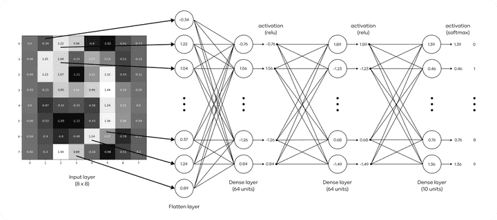
Now that our data is ready, we define the structure of the MLP. We use TensorFlow’s Keras API to create a simple neural network model with the following architecture:
- Input Layer: 64 nodes (corresponding to the 64 pixels in each image).
- Hidden Layer 1: 64 neurons with the
ReLUactivation function. - Hidden Layer 2: 64 neurons with the
ReLUactivation function. - Output Layer: 10 neurons (one for each digit), with a
softmaxactivation function to output probabilities for each class.
from tensorflow.keras.models import Sequential
from tensorflow.keras.layers import Dense

model = Sequential([
    Dense(64, activation='relu', input_shape=(X_train.shape[1],)),
    Dense(64, activation='relu'),
    Dense(10, activation='softmax')
])
The choice of ReLU (Rectified Linear Unit) is common because it helps mitigate the vanishing gradient problem and allows the network to learn complex patterns.
⚙️ Compiling and Training the Model
The model is compiled using the adam optimizer and categorical_crossentropy as the loss function, which is ideal for multi-class classification tasks. We also track accuracy during training.
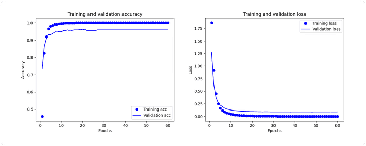
model.compile(optimizer='adam', loss='categorical_crossentropy', metrics=['accuracy'])We then train the model for 60 epochs, with 20% of the training data used for validation. During training, the model adjusts its weights to minimize the loss function.
history = model.fit(X_train, y_train, epochs=60, validation_split=0.2)🎓 Evaluating Model Performance
After training, we evaluate the model on the test set to see how well it generalizes to unseen data.
loss, accuracy = model.evaluate(X_test, y_test)
print(f"Test Accuracy: {accuracy*100:.2f}%")
Additionally, we can generate predictions and assess performance using metrics like accuracy and a classification report:
from sklearn.metrics import accuracy_score, classification_report
import numpy as np

y_pred = np.argmax(model.predict(X_test), axis=1)
y_test_numeric = np.argmax(y_test, axis=1)

accuracy = accuracy_score(y_test_numeric, y_pred)
print(f"Accuracy: {accuracy}")
print(f"Classification report:
{classification_report(y_test_numeric, y_pred)}")
Accuracy: 0.975
Classification report:
precision recall f1-score support
0 1.00 1.00 1.00 33
1 0.97 1.00 0.98 28
2 0.97 0.97 0.97 33
3 0.97 0.94 0.96 34
4 1.00 1.00 1.00 46
5 0.96 0.98 0.97 47
6 0.97 0.97 0.97 35
7 1.00 0.97 0.99 34
8 0.94 0.97 0.95 30
9 0.97 0.95 0.96 40
accuracy 0.97 360
macro avg 0.97 0.97 0.97 360
weighted avg 0.98 0.97 0.98 360🔎 Visualizing Training Progress
To understand the model’s training progress, we can plot the loss and accuracy curves over the epochs:
import matplotlib.pyplot as plt

history_dict = history.history
epochs = range(1, len(history_dict['accuracy']) + 1)

# Plot loss
plt.plot(epochs, history_dict['loss'], 'bo', label='Training loss')
plt.plot(epochs, history_dict['val_loss'], 'b', label='Validation loss')
plt.title('Training and validation loss')
plt.xlabel('Epochs')
plt.ylabel('Loss')
plt.legend()
plt.show()

# Plot accuracy
plt.plot(epochs, history_dict['accuracy'], 'bo', label='Training accuracy')
plt.plot(epochs, history_dict['val_accuracy'], 'b', label='Validation accuracy')
plt.title('Training and validation accuracy')
plt.xlabel('Epochs')
plt.ylabel('Accuracy')
plt.legend()
plt.show()
🎉 Conclusion
In this article, we’ve walked through the process of building an MLP for handwritten digit recognition. By preprocessing the data, constructing an MLP model with two hidden layers, and using techniques like ReLU activation and softmax for classification, we’ve achieved an effective solution for this classic machine learning problem.

Feel free to modify this model by experimenting with different architectures, activation functions, or optimization techniques!