Iris Dataset Clustering with K-Means: A Step-by-Step Analysis

Clustering is one of the core techniques in unsupervised learning. It enables us to group similar data points without requiring any predefined labels. In this article, we explore how the K-Means algorithm can be applied to the widely-used Iris dataset, focusing on the sepal features.
The objective of this analysis is to illustrate the entire clustering process, from determining the optimal number of clusters using the Elbow method to applying K-Means and comparing the results with the original data.
📊 Dataset : Iris

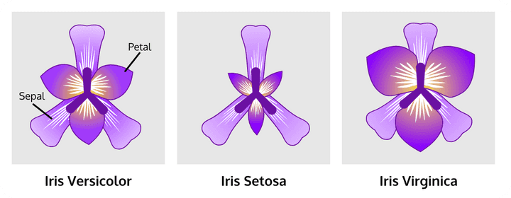
The Iris dataset contains 150 samples of iris flowers, each described by four features: sepal length, sepal width, petal length, and petal width. For this analysis, we focus on the sepal length and sepal width features to implement K-Means.
💭 What is K-Means Clustering?
K-Means is an algorithm that partitions a dataset into K distinct clusters. The basic idea is to assign each data point to the cluster whose centroid is closest to it. The algorithm seeks to minimize the inertia of the clusters.
-
Centroid: The centroid is the “mean” or center point of all the data points in a cluster. For each cluster, K-Means calculates the centroid, and each point is assigned to the cluster with the nearest centroid.
Mathematically, for a cluster Cj, the centroid μj is calculated as:

This formula simply means that the centroid is the average of all the data points x in the cluster Cj.
-
Inertia: Inertia measures how spread out the clusters are. It is the sum of the squared distances between each data point and its assigned cluster’s centroid. A lower inertia means the data points are closer to the centroids, indicating well-defined clusters.
The inertia is computed as:

This formula sums up the squared distances between each point x and the centroid μj of its cluster. The goal of K-Means is to minimize this inertia.
🔎 Loading and Visualizing the Data
First, we load the Iris dataset and visualize the sepal features without any clustering to understand the data in its raw form.
# Load the Iris dataset
iris = load_iris()
df_iris = pd.DataFrame(iris.data, columns=iris.feature_names)
df_iris['target'] = iris.target
🔭 Plot the Original Dataset
We plot the original dataset (without clustering) to show how the sepal features are distributed in their raw form.
# Plot the original dataset for comparison (without clustering and centroids)
plt.figure(figsize=(10, 7))
sns.scatterplot(x=df_iris['sepal length (cm)'], y=df_iris['sepal width (cm)'],
                color='gray', s=150, edgecolor='black', linewidth=1.5)
plt.title('Original Iris Dataset (Sepal Features)', fontsize=16)
plt.xlabel('Sepal Length (cm)', fontsize=14)
plt.ylabel('Sepal Width (cm)')
plt.grid(True)
plt.show()
⚖️ Standardizing the Data
Since K-Means is sensitive to the scale of the data, we standardize the features using StandardScaler. This ensures that each feature contributes equally to the clustering process.
# Standardize the features
scaler = StandardScaler()
df_iris_scaled = scaler.fit_transform(df_iris.drop('target', axis=1))
💪 The Elbow Method for Optimal Clustering
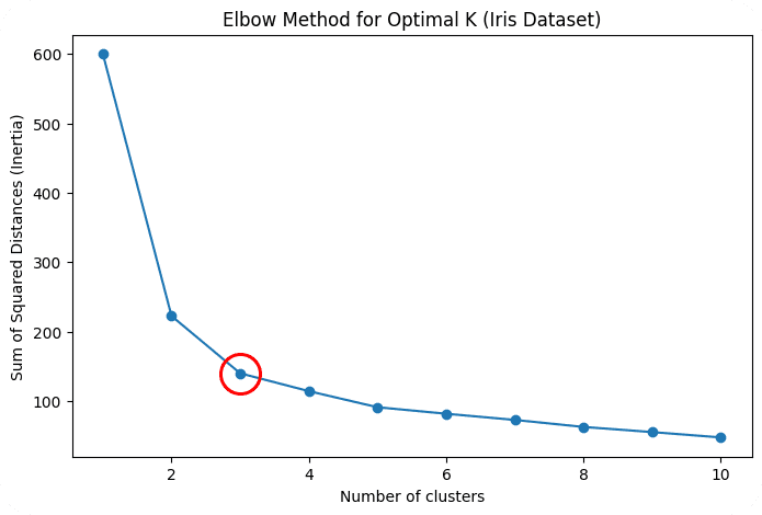
One of the most important decisions in K-Means is determining the number of clusters K. A common approach is the Elbow Method. This method involves plotting the inertia for different values of K. As we increase K, the inertia decreases because clusters become smaller. However, after a certain point, the reduction in inertia slows down, forming an “elbow” in the graph. This point is considered the optimal number of clusters.
# Elbow method to find the optimal number of clusters
sse_iris = []
for k in range(1, 11):
    kmeans = KMeans(n_clusters=k, random_state=42)
    kmeans.fit(df_iris_scaled)
    sse_iris.append(kmeans.inertia_)

plt.figure(figsize=(8, 5))
plt.plot(range(1, 11), sse_iris, marker='o')
plt.title('Elbow Method for Optimal K (Iris Dataset)')
plt.xlabel('Number of clusters')
plt.ylabel('Sum of Squared Distances (Inertia)')
plt.show()
In this case, the elbow occurs around K = 3, which indicates that three clusters are optimal for this dataset.
3️⃣ Applying K-Means with K = 3
Once we determine K = 3 as the optimal number of clusters, we apply K-Means and assign each data point to its corresponding cluster.
# Apply K-Means with optimal K (K = 3)
kmeans_iris = KMeans(n_clusters=3, random_state=42)
df_iris['Cluster'] = kmeans_iris.fit_predict(df_iris_scaled)
👀 Visualizing the Clusters and Centroids
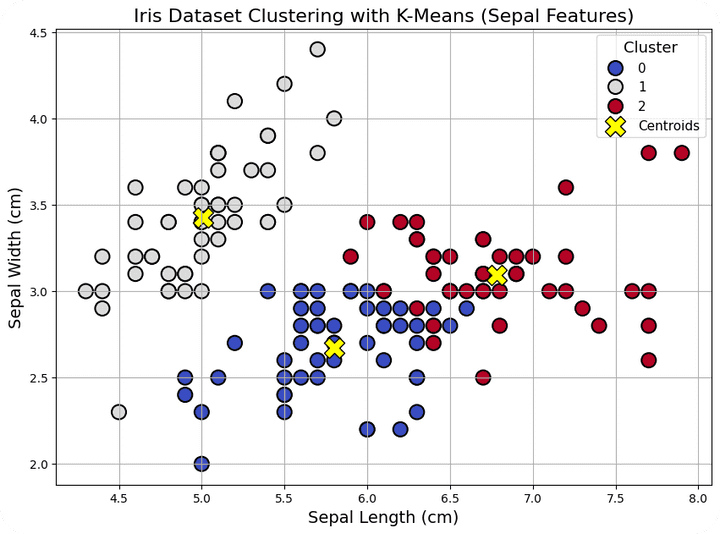
Finally, we visualize the clustered data. We use sepal length and sepal width as axes and plot the data points color-coded by their cluster. We also plot the centroids of each cluster, which are the mean values of all points in the cluster.
Since the K-Means algorithm was applied on standardized data, the centroids were initially calculated on the scaled features. To display the centroids correctly in the original feature space (with sepal length and sepal width), we needed to inverse transform the centroid coordinates back to their original scale. This step ensures that the centroids are properly aligned with the clusters on the graph.
# Visualize the clusters using 'sepal length' and 'sepal width'
plt.figure(figsize=(10, 7))
sns.scatterplot(x=df_iris['sepal length (cm)'], y=df_iris['sepal width (cm)'],
                hue=df_iris['Cluster'], palette='coolwarm', s=150, edgecolor='black', linewidth=1.5)
plt.title('Iris Dataset Clustering with K-Means (Sepal Features)', fontsize=16)
plt.xlabel('Sepal Length (cm)', fontsize=14)
plt.ylabel('Sepal Width (cm)', fontsize=14)
plt.grid(True)

# Correctly transform centroids back to the original scale
centroids_original = scaler.inverse_transform(kmeans_iris.cluster_centers_)

# Plot centroids in the original scale
plt.scatter(centroids_original[:, 0], centroids_original[:, 1], s=300, c='yellow', label='Centroids', edgecolor='black', marker='X')
plt.legend(title='Cluster', title_fontsize='13', fontsize='11', loc='upper right')
plt.show()
✅ Conclusion
Through this analysis, we have demonstrated how to apply K-Means clustering to the Iris dataset, with a focus on sepal length and sepal width. We explained key concepts like centroids, inertia, and the Elbow Method to select the optimal number of clusters. By visualizing the clustered data and comparing it to the original dataset, we saw how K-Means effectively partitions data into well-defined groups.
In future articles, we will explore other machine learning techniques and apply them to different datasets to uncover hidden patterns.